Global Plastic Pollution Analysis with Machine Learning

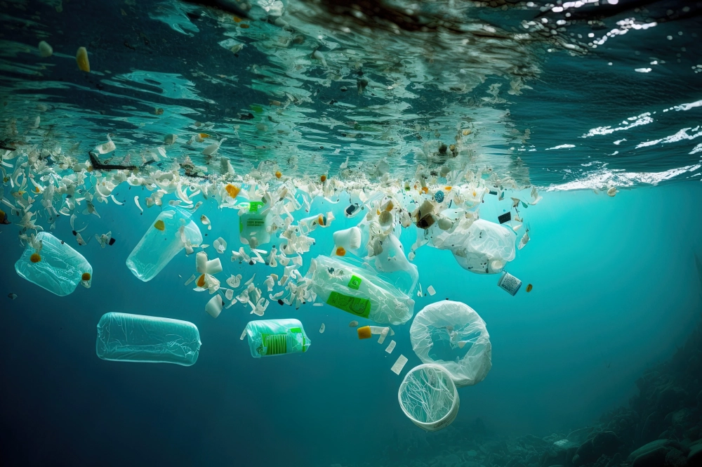
In the battle against global plastic pollution, data-driven insights are crucial for understanding its extent, identifying hotspots, and devising effective mitigation strategies. Leveraging the power of machine learning, we embark on a journey to analyze and interpret vast datasets related to plastic pollution worldwide. In this article, we explore how machine learning algorithms can uncover valuable insights into the distribution, trends, and environmental impact of plastic pollution, paving the way for informed decision-making and sustainable solutions.

1. Data Acquisition and Preprocessing:To kickstart our analysis, we gather diverse datasets encompassing information on plastic waste production, consumption patterns, recycling rates, pollution levels, and environmental factors. Through rigorous preprocessing steps including cleaning, normalization, and feature engineering, we ensure the quality and relevance of the data for model training and analysis.


2. Exploratory Data Analysis (EDA):With our datasets prepared, we delve into exploratory data analysis to gain a deeper understanding of the patterns and trends underlying global plastic pollution. Through visualizations, statistical analyses, and spatial mapping techniques, we uncover key insights such as the geographic distribution of plastic pollution, temporal trends in waste generation, and correlations with socio-economic indicators.


3. Model Training and Evaluation:Next, we employ machine learning algorithms to build predictive models that can analyze and forecast plastic pollution levels based on various input variables. Using supervised learning techniques such as regression and classification, we train models to predict pollution levels in different regions, identify contributing factors, and assess the effectiveness of potential interventions. Model performance is evaluated using metrics such as accuracy, precision, recall, and F1-score to ensure reliability and robustness.


4. Interpretation and Insights:Through model interpretation techniques such as feature importance analysis and SHAP (SHapley Additive exPlanations), we gain insights into the factors driving plastic pollution and their relative importance. These insights can inform policy decisions, urban planning, waste management strategies, and public awareness campaigns aimed at reducing plastic consumption and promoting recycling initiatives.


5. Future Directions and Impact:As we continue to refine our analysis and models, the insights gleaned from our global plastic pollution analysis have the potential to drive meaningful change and policy action at local, national, and international levels. By harnessing the power of machine learning to understand, quantify, and address plastic pollution, we can work towards a cleaner, healthier planet for future generations.

Download the data-set from the download link and run the code in google colab to train your model.

The below code is .Python file.

# %%
import numpy as np 
import pandas as pd 
import seaborn as sns 
import warnings
import matplotlib.pyplot as plt 
%matplotlib inline 

warnings.filterwarnings('ignore')
sns.set_style('darkgrid')

# %%
''' reading dataset '''
df = pd.read_csv('per-capita-plastic-waste-vs-gdp-per-capita.csv')

# %%
''' displaying first 5 rows '''
df.head()

# %%
''' shape of data '''
df.shape

# %%
''' checking null values in data '''
df.isnull().sum()

# %%
''' checking percentage of null values in each column '''
for column in df.columns:
    print("{} has {:.2f}% null values: ".format(column, (df[column].isnull().sum() / len(df)) * 100 ))
    print("-" * 100)

# %%
''' checking info of data '''
df.info()

# %%
''' renaming column names '''
df.rename(columns={'GDP per capita, PPP (constant 2011 international $)': 'GDP per capita in PPP', 
                   'Total population (Gapminder, HYDE & UN)': 'Total Population',
                    'Per capita plastic waste (kg/person/day)': 'Waste per person(kg/day)'}, inplace=True)

# %%
df.head()

# %%
''' removing entities/countries with incomplete/missing data '''
incmp_df_idx = df[(df['Total Population'].isna()) & (df['GDP per capita in PPP'].isna())].index
df.drop(incmp_df_idx, inplace=True)

# %%
df.head()

# %%
df.shape

# %%
'''retrieving rows in which year == 2010'''
df_2010 = df[df['Year'] == 2010]
df_2010 = df_2010.drop(columns='Continent')

# %%
df_2010.head()

# %%
'''retrieving continent name in which year == 2015'''
df_2015 = df[df['Year'] == 2015]
df_2010['Continent'] = df_2015['Continent'].values

# %%
df_2015.head()

# %%
'''dropping rows with missing Continent values using index'''
missing_idx = df_2010[df_2010['Continent'].isna()].index
df_2010.drop(missing_idx, inplace=True)

# %%
''' dropping rows with missing per person waste generation values '''
df_2010 = df_2010[df_2010['Waste per person(kg/day)'].notna()]
wa_g = df_2010.reset_index().drop('index', axis=1)

# %%
wa_g.head()

# %%
''' reading 2nd file '''
df2 = pd.read_csv('per-capita-mismanaged-plastic-waste-vs-gdp-per-capita.csv')

# %%
''' displaying first 5 rows of df2 '''
df2.head()

# %%
''' renaming columns'''
df2.rename(columns={'Per capita mismanaged plastic waste': 'Mismanaged waste per person(kg/day)',
                  'GDP per capita, PPP (constant 2011 international $)': 'GDP per capita in PPP',
                  'Total population (Gapminder, HYDE & UN)': 'Total Population'}, inplace=True)

# %%
''' dropping Continent column '''
df2.drop('Continent', axis=1, inplace=True)

# %%
'''retrieving rows in which year == 2010'''
df2_2010 = df2[df2.Year == 2010]
df2_2010.head()

# %%
''' dropping rows with missing mismanaged waste values '''
df2_2010 = df2_2010[df2_2010['Mismanaged waste per person(kg/day)'].isna() != True]

''' reset index '''
w_m = df2_2010.reset_index().drop('index', axis=1)

# %%
w_m.head()

# %%
''' merging w_m and wa_g '''
df_plastic_waste = pd.merge(wa_g, w_m, how='inner')

# %%
''' displaying data '''
df_plastic_waste.head()

# %%
''' converting column names into list '''
df_plastic_waste.columns.tolist()

''' column names '''
col_names = ['Entity','Code','Year','Waste per person(kg/day)','Mismanaged waste per person(kg/day)',
           'GDP per capita in PPP','Total Population','Continent']

df_plastic_waste = df_plastic_waste[col_names]

'''rounding the values per person'''
df_plastic_waste.iloc[:, 3:5] = np.around(df_plastic_waste[['Waste per person(kg/day)', 
                                                            'Mismanaged waste per person(kg/day)']], decimals=2)

''' changing data type '''
df_plastic_waste['Total Population'] = df_plastic_waste['Total Population'].astype(int)

# %%
'''Generating Total waste and Total mismanaged waste by country'''
df_plastic_waste['Total waste(kgs/year)'] = ((df_plastic_waste['Waste per person(kg/day)'] * 
                                    df_plastic_waste['Total Population']) * 365)
df_plastic_waste['Total waste mismanaged(kgs/year)'] = ((df_plastic_waste['Mismanaged waste per person(kg/day)'] * 
                                    df_plastic_waste['Total Population']) * 365)

# %%
df_plastic_waste.head()

# %%
''' scatter plot graph '''

plt.figure(1, figsize=(12,8))
plt.scatter(df_plastic_waste['GDP per capita in PPP'], df_plastic_waste['Mismanaged waste per person(kg/day)'])
plt.title('Waste Mismanaged', loc='center', fontsize=15)
plt.ylabel('Mismanaged waste', loc='center', fontsize=15)
plt.xlabel('GDP per capita', fontsize=12)

sns.regplot(x='GDP per capita in PPP', y='Mismanaged waste per person(kg/day)', data=df_plastic_waste,
           scatter_kws={'color': '#34568B'}, line_kws={'color': '#650021'})

plt.show()

# %%
''' scatter plot '''

plt.figure(2, figsize=(12,8))
plt.scatter(df_plastic_waste['GDP per capita in PPP'], df_plastic_waste['Waste per person(kg/day)'])
plt.title('Waste Generated by GDP', loc='center', fontsize=14)
plt.ylabel('Waste per person(kg/day)', loc='center', fontsize=12)
plt.xlabel('GDP per capita in PPP', fontsize=12)

sns.regplot(x=df_plastic_waste['GDP per capita in PPP'], y=df_plastic_waste['Waste per person(kg/day)'],
           scatter_kws={'color': '#CD212A'}, line_kws={'color': '#380282'})

plt.show()

# %%

Conclusion

In conclusion, the application of machine learning in the analysis of global plastic pollution offers unprecedented opportunities to uncover hidden patterns, predict future trends, and inform evidence-based decision-making. By harnessing the vast potential of data-driven insights, we can work collaboratively towards mitigating the environmental impact of plastic pollution and preserving the health of our planet for generations to come.

"Stay tuned for future data science projects that will turbocharge your learning journey and take your skills to the next level!"